FINIST POWER SYSTEM MODEL
INTRODUCTION
The feature that truly sets FINIST apart is its power system model calculation. Traditional operator training simulators often model the operation of the electric power system as a sequence of steady states. More sophisticated ones may model transitional and dynamic processes that result from a disturbance. However, there is always an assumption that the system reaches a steady state before the occurrence of the next disturbance or other external event. Such an approach significantly simplifies the simulator design as there is no need to consider the next disturbance while the effects of the previous one are still being computed. However, such simplification sacrifices the realism of the power system operation and diminishes the usefulness of such simulator for operator training.
FINIST takes a radically different approach to power system modeling. FINIST continuously models the system dynamics and processes the effect of external events as they happen. Instead of forcing the system into a steady state, FINIST periodically computes the state and powerflow of the system to be exported to its clients as it continues to calculate the system dynamics.
The choice of this sophisticated model places additional demands on the efficiency of the model calculation as the dynamics of the system regardless of its scale, has to be computed in real-time. In fact, if the simulation time is accelerated, the model has to be computed even faster. FINIST successfully meets these performance expectations.
COMPUTATION ALGORITHM OUTLINE
FINIST's model computation algorithm is shown below. The computation is iterative. Each iteration computes a fixed simulated time period. By default, the length of this time period is 200 ms. The processing of each period starts with simulation time adjustment. The computation engine then inputs the external events that occur during the new time period.
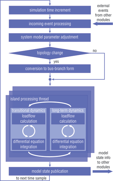
Some of the events, such as closing a breaker or grounding a bus, change system topology. After each topology change, the topology processor of the computation engine converts the system into a bus-branch model by collapsing each portion of the system with zero impedance (such as bus segments connected by a closed breaker) into a single computational node. The computation engine then determines electrically independent islands and proceeds to compute the dynamics for each island. FINIST is fully capable of modeling the power system that consists of several islands. The simulator can handle rather sophisticated cases such as when the generators of the same power plant are electrically separated into several islands.
After the dynamics for the specified time period has been computed, the computation engine calculates and publishes the resultant system powerflow for other modules and external programs to use and moves to the next time period. The powerflow publication can proceed concurrently with the next time period computation. In effect, FINIST continuously processes the dynamics of the power system periodically importing external events and publishing the powerflow.
ISLAND DYNAMICS CALCULATION
The computation engine calculates the dynamics for each island concurrently. There is a separate thread for each island. For computational efficiency, the simulated time can flow at different rate in each island. However, these simulated time flows are periodically aligned for all islands. This alignment enables taking global system state snapshots for the purposes of publishing the complete system powerflow. The default alignment period is 200 ms.
Depending on the speed of the simulated processes occurring in each island, FINIST models them as transitional processes or as (long-term) dynamic processes. These two computation models in FINIST are different. However, FINIST can switch between the models as needed. Synchronous machines, specifically generators, are the major objects of dynamic processes modeling. Certain control systems, such as automatic generation control (AGC), are also treated as dynamic system elements. The two computation models place different assumptions on the behavior of these objects.
In case of long-term dynamics model, some of the fast electromechanical processes are not significant. Therefore, they are not taken into account. In this model, FINIST assumes that the rotors of all synchronous machines rotate with the same speed. FINIST does not consider delays in generator excitation systems or the transitional processes in the generator armature. FINIST determines rotor acceleration by using system powerflow calculation: the power used to accelerate the rotor of a synchronous machine attached to a certain bus is considered as one of the components of power balance of this bus. FINIST computes the island frequency by integrating the rotor acceleration of the synchronous machines of the island. In this model FINIST computes prime mover dynamics of the power plants.
FINIST uses transitional process model to represent electromechanical phenomena that occur in power systems after topology change or during loss of synchronism. Such processes develop fast and require a significantly more detailed model. In this model, FINIST factors in the changes of generator rotor angles, the excitation system inertia, as well as transitional processes in the generator's electromagnetic circuits. Also in this model, the acceleration of each individual rotor is another state variable to be computed. The synchronous machines are represented in the form of subtransient EMF and subtransient impedance.
The power system processes are modeled as a system of differential and algebraic equations. The differential equations are solved by time step integration. In a single integration step, the system parameters are assumed to be fixed and the algebraic equations are solved to obtain the powerflow: the voltage magnitude and angle for each node. The length of a step and thus frequency of state calculation depends on the particular dynamics model.
POWERFLOW CALCULATION
The challenge of powerflow calculation is to ensure its convergence. FINIST switches between the transitional process and long-term dynamics model as needed. The transitional process model is used after topology change or if the long term dynamic computation does not converge. The lack of convergence usually signifies the lack of dynamic stability which leads to the loss of generator synchronism. FINIST switches back to long-term dynamics model when the difference between speed and acceleration of the synchronous machines falls below certain thresholds.
The powerflow calculation in transitional process and long-term dynamics model differs. The objective of long-term dynamics powerflow calculation is to provide adequate fidelity and fast state processing. The objective of transitional process calculation is to ensure convergence. FINIST ensures the overall convergence of the powerflow computation by switching between models. For example, if the system is in or near loss of synchronism, the powerflow calculation in long-term dynamics model may not converge. If the long-term dynamics model does not converge, FINIST switches to transitional process dynamics whose convergence is guaranteed.
In long-term dynamics model, FINIST computes bus voltages using Gauss-Newton minimization method possibly augmented with Siedel iterations for fast convergence. The basic algorithms are enhanced with a number of optimization techniques. FINIST implements integration step-size adjustment. FINIST has protection against jitter caused by a generator operating near its reactive power supply limit and alternating between voltage level regulation mode and reactive power limitaion mode. FINIST allows flat start or a start from some pre-defined state.
FINIST can use one of the several methods of balancing the powerflow calculation: with one or several slack busses and set frequency; with distributed slack bus and set frequency; with generator governor adjustment and the effect of load on frequency. If the system is separated into several islands FINIST can apply different balancing methods to different islands.
FINIST uses Z-method to compute powerflow in transitional process model. Each load is divided into two parts that are related to: (i) load admittance and (ii) current injected into the system. The load admittance is considered constant during the iterations of the powerflow calculations. Moreover, the load admittance is fixed across several adjacent integration steps of the differential equations solution. The current, on the other hand, is computed according to the load sensitivity function. It is re-computed in every iteration. This approach has good convergence properties. In rare cases, Z-method may not converge fast enough at a particular integration step. Then, the load admittance is recalculated and the powerflow calculation is repeated. In case the method still does not converge, the load admittance is fixed. The powerflow then devolves to directly solving a system of linear equations. That is, the powerflow calculation in FINIST's transitional process model always converges.
DIFFERENTIAL EQUATION SOLUTIONS
In long-term dynamics model, FINIST uses explicit multi-step predictor-corrector variable-order method derived from Adams method. The method considers the stiffness of the differential equations. The integration step size is selected individually for each step. Proportional-integral law is used for step selection. Specifically, the step size is selected such that the logarithms of the three adjacent steps constitute a second order linear differential equation to be solved explicitly. For every step, the coefficients for such an equation are adjusted based on the predicted and computed values. This step size control allows FINIST to optimize the step size, eliminate unnecessarily frequent small step recalculations, and thus speed up the overall calculations. Even though step sizes in each island may be different, the integration computations at each island periodically synchronize. The duration of this period is fixed and is significantly larger than integration step sizes. By default it is set to 200 ms.
This synchronization allows FINIST to determine the state of the complete system and publish it for the external programs.
Different groups of state variables are integrated using either explicit or implicit methods. Implicit methods result in increased step size which speeds up the computation without numerical stability loss. They are used for simulating stiff dynamics. Explicit methods are used for the simulation of generating units with slow dynamics such as thermal or nuclear generators.
In transitional process model, FINIST uses diagonal Runge-Kutta method to solve the set differential equations. The step size for this method is fixed. By default it is set to 20 ms. The second order of this method has an optimal combination of speed and reliability of convergence.